Where US‑67 can be seen from the Viewing Area
A 0.66 m headlamp on US‑67 between Shafter and Marfa, tested for terrain occlusion from an eye 1.6 m above the viewing platform. Earth curvature (exact, on the WGS84 ellipsoid) and atmospheric refraction are included. Terrain is USGS 1-metre lidar, with shrubs and structures from the lidar point cloud.
The 120° viewing fan
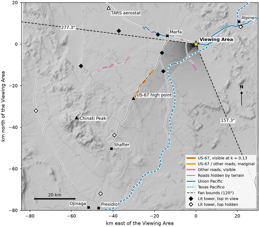
Standard atmosphere, k = 0.13
The textbook refraction state. Each 60 m of road is classed by whether a headlight clears the terrain in between.
- Visible, clears distant terrain by more than 5 m
- Marginal, depends on sub-metre detail (grass, eye height)
- Hidden by terrain
- Texas Pacifico railroad
Across refraction states
Colour is the smallest refraction coefficient k at which a headlight becomes visible. Night surface inversions raise k; daytime heating lowers it.
What the platform sees, looking southwest to west
Apparent elevation angle against true azimuth, at standard refraction. The shaded ground ends at the modelled skyline, which along most of this arc is the Chinati Mountains 60–70 km away. Visible road points sit below that skyline, so their headlights appear against dark mountainside rather than open sky. Hidden points are drawn faintly where they would appear if the nearer ground were not in the way. This frame is built for overlaying on calibrated photos later. 1 mrad ≈ 0.057°, about a car length at 80 m.
- Visible
- Marginal
- Hidden
- Skyline (k = 0.13)
Three sight lines, drawn with curvature
Terrain height relative to the observer's eye, after the curvature-and-refraction drop. A straight line from the eye to the car is the line of sight. Solid is standard refraction. Dashed is a strong inversion (k = 0.5), which lifts distant terrain less and flattens the Earth optically.
Visible stretches at standard refraction, as a table
| Stretch | Chainage km | Azimuth ° | Distance km | Road elev m | Apparent elev mrad | Length m |
|---|
How it was computed
- US‑67 is the TxDOT centreline, resampled every 60 m, with 1,075 points from Shafter (km 0) to the US-90 junction in Marfa (km 64.4). (The author's Google Earth trace agrees with it to 2 m, median.)
- For each point, terrain is sampled along the WGS84 geodesic from the viewer, every 2 m within 3 km of either end and every 5 m in between, from the 1 m lidar DEM (1/3″ and 1″ DEMs beyond it). Eye, lamp and ground are placed in Earth-centred coordinates, with heights converted by the GEOID12B geoid model.
- Refraction bends the ray into an arc above the straight eye–lamp chord. The visibility threshold kcrit is solved in closed form and tested against brute force; 22 unit tests cover the engine.
- Only the first 5 m (the observer) and the last 3 m (the car itself) are skipped: the lidar resolves the road bed. Classes come from a Monte Carlo over lidar error and eye height: visible means seen in at least 95% of draws and still seen under 0.25 m of grass; hidden means seen in at most 5%.
What limits it
- Constant k. Near-ground gradients vary strongly with height. Hirt et al. measured k from about −4 by day to +16 near sunset at 1.8 m. Ray tracing through assumed night-time temperature layers adds at most about 1.5 km of visible road and lifts lights by up to 0.12°; the real profile still has to be measured.
- Humidity barely bends visible light. The water-vapour term in the optical refractive index is small (Ciddor 1996). Humidity matters here mainly through haze and extinction, which dims lights. It does not change what is occluded.
- Grass. The lidar resolves shrubs and structures but not grass shorter than about 0.3 m; allowing 0.25 m of grass everywhere removes about 0.5 km of visible road.
- Headlights are directional. This model says where a lamp is geometrically visible, not whether it points at you. Road heading is the next layer.